After having read the first part of a Rcpp tutorial which compared native R vs C++ implementations of a Fibonacci sequence generator, I resorted to drawing the so-called Golden Spiral using R.

Libraries used in this example are the following

library(ggplot2)
library(plotrix)

In polar coordinates, this special instance of a logarithmic spiral's functional representation can be simplified to r(t) = e^(0.0635*t) For every quarter turn, the corresponding point on the spiral is a factor of phi further from the origin (r is this distance), with phi the golden ratio - the same one obtained from dividing any 2 sufficiently big successive numbers on a Fibonacci sequence, which is how the golden ratio, the golden spiral and Fibonacci sequences are linked concepts!

polar_golden_spiral <- function(theta) exp(0.30635*theta)

Let's do 2 full circles. First, I create a sequence of angle values theta. Since 2 * PI is the equivalent of a circle in polar coordinates, we need to have distances from origin for values between 0 and 4 * PI.

seq_theta <- seq(0,4*pi,by=0.05)

dist_from_origin <- sapply(seq_theta,polar_golden_spiral)

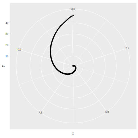
Plotting the function using coord_polar in ggplot2 does not work as intended. Unexpectedly, the x axis keeps extending instead of circling back once a full circle is reached. Turns out coord_polar might not really be intended to plot elements in polar vector format.

ggplot(data.frame(x = seq_theta, y = dist_from_origin), aes(x,y)) +
    geom_point() +
    coord_polar(theta="x")

To ensure what I was trying to do is possible, I employ a specialised plotfunction instead

plotrix::radial.plot(dist_from_origin, seq_theta,rp.type="s", point.col = "blue")

With that established and the original objective of the exercise achieved, it still would be nice to be able to accomplish this using ggplot2. To do so, the created sequence above needs to be converted to cartesian coordinates. The rectangular function equivalent of the golden spiral function r(t) defined above is a(t) = (r(t) cos(t), r(t) sin(t)) It's not too hard to come up with a hack to convert one to the other.

cartesian_golden_spiral <- function(theta) {
    a <- polar_golden_spiral(theta)*cos(theta)
    b <- polar_golden_spiral(theta)*sin(theta)
    c(a,b)
}

Applying that function to the same series of angles from above and stitching the resulting coordinates in a data frame. Note I'm enclosing the first expression in brackets, which prints it immediately, which is useful when the script is run interactively.

(serie <- sapply(seq_theta,cartesian_golden_spiral))
df <- data.frame(t(serie))

With everything now ready in the right coordinate system, it's now only a matter of setting some options to make the output look acceptable.

ggplot(df, aes(x=X1,y=X2)) +
    geom_path(color="blue") +
    theme(panel.grid.minor = element_blank(),
          axis.text.x = element_blank(),
          axis.text.y = element_blank()) +
    scale_y_continuous(breaks = seq(-20,20,by=10)) +
    scale_x_continuous(breaks = seq(-20,50,by=10)) +
    coord_fixed() +
    labs(title = "Golden spiral",
         subtitle = "Another view on the Fibonacci sequence",
         caption = "Maths from https://www.intmath.com/blog/mathematics/golden-spiral-6512\nCode errors mine.",
         x = "",
         y = "")

Note on how this post was written: After a long hiatus, I set about using emacs, org-mode and ESS together to create this post. All code is part of an .org file, and gets exported to markdown using the orgmode conversion - C-c C-e m m.