Recently inspired to doing a little analysis again, I landed on a dataset from https://bitre.gov.au/statistics/safety/fatal_road_crash_database.aspx, which I downloaded on 5 Oct 2017. Having open datasets for data is a great example of how governments are moving with the times!
Trends
I started by looking at the trends - what is the approximate number of road fatalities a year, and how is it evolving over time? Are there any differences noticeable between states? Or by gender?
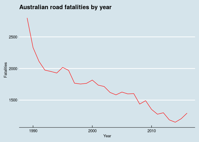
Figure 1: Overall trendline
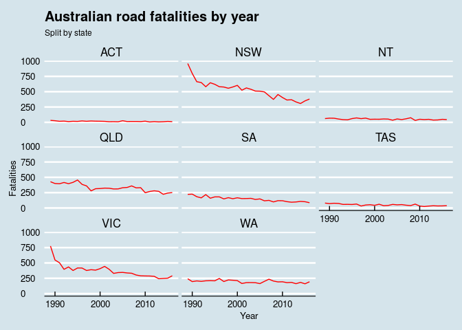
Figure 2: Trendlines by Australian state
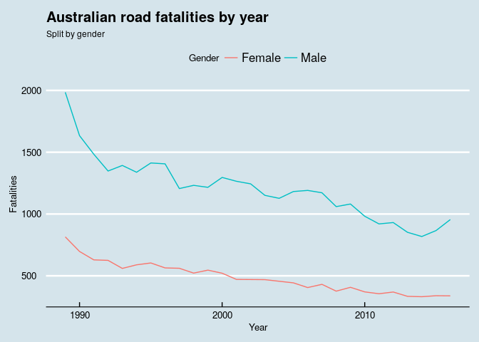
Figure 3: Trendlines by gender
What age group is most at risk in city traffic?
Next, I wondered if there were any particular ages that were more at risk in city traffic. I opted to quickly bin the data to produce a histogram.
fatalities %>%
  filter(Year != 2017, Speed_Limit <= 50) %>%
  ggplot(aes(x=Age))+
  geom_histogram(binwidth = 5) +
  labs(title = "Australian road fatalities by age group",
       y = "Fatalities") +
  theme_economist()

## Warning: Removed 2 rows containing non-finite values (stat_bin).
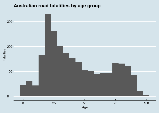
Figure 4: histogram
Hypothesis
Based on the above, I wondered - are people above 65 more likely to die in slow traffic areas? To make this a bit easier, I added two variables to the dataset - one splitting people in younger and older than 65, and one based on the speed limit in the area of the crash being under or above 50 km per hour - city traffic or faster in Australia.
fatalities.pensioners <- fatalities %>%
  filter(Speed_Limit <= 110) %>% # less than 2% has this - determine why
  mutate(Pensioner = if_else(Age >= 65, TRUE, FALSE)) %>%
  mutate(Slow_Traffic = ifelse(Speed_Limit <= 50, TRUE, FALSE)) %>%
  filter(!is.na(Pensioner))
To answer the question, I produce a density plot and a boxplot.
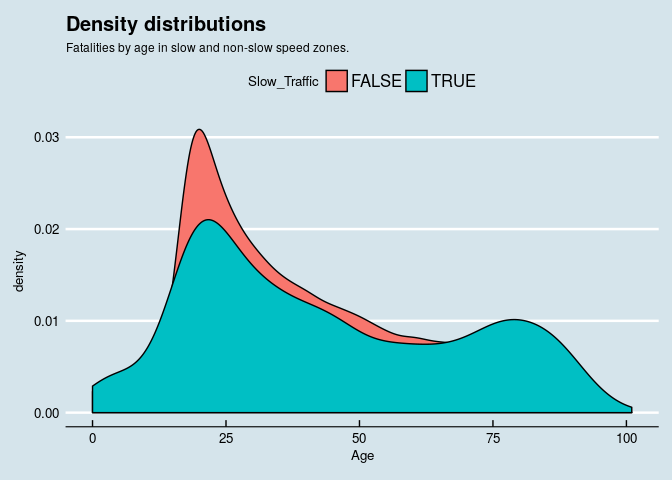
Figure 5: densityplot
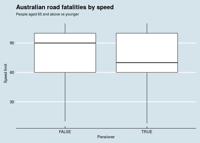
Figure 6: boxplot
Some further statistical analysis does confirm the hypothesis!
# Build a contingency table and perform prop test
cont.table <- table(select(fatalities.pensioners, Slow_Traffic, Pensioner))
cont.table

##             Pensioner
## Slow_Traffic FALSE  TRUE
##        FALSE 36706  7245
##        TRUE   1985   690

prop.test(cont.table)

##
##  2-sample test for equality of proportions with continuity
##  correction
##
## data:  cont.table
## X-squared = 154.11, df = 1, p-value < 2.2e-16
## alternative hypothesis: two.sided
## 95 percent confidence interval:
##  0.07596463 0.11023789
## sample estimates:
##    prop 1    prop 2
## 0.8351573 0.7420561

# Alternative approach to using prop test
pensioners <- c(nrow(filter(fatalities.pensioners, Slow_Traffic == TRUE, Pensioner == TRUE)), nrow(filter(fatalities.pensioners, Slow_Traffic == FALSE, Pensioner == TRUE)))
everyone <- c(nrow(filter(fatalities.pensioners, Slow_Traffic == TRUE)), nrow(filter(fatalities.pensioners, Slow_Traffic == FALSE)))
prop.test(pensioners,everyone)

##
##  2-sample test for equality of proportions with continuity
##  correction
##
## data:  pensioners out of everyone
## X-squared = 154.11, df = 1, p-value < 2.2e-16
## alternative hypothesis: two.sided
## 95 percent confidence interval:
##  0.07596463 0.11023789
## sample estimates:
##    prop 1    prop 2
## 0.2579439 0.1648427
Conclusion
It's possible to conclude older people are over-represented in the fatalities in lower speed zones. Further ideas for investigation are understanding the impact of the driving age limit on the fatalities - the position in the car of the fatalities (driver or passenger) was not yet considered in this quick look at the contents of the dataset.
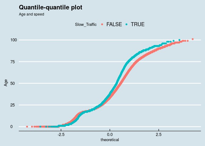
Figure 7: quantile-quantile plot
Posted on Tuesday 10 October 2017 at 16:56